Specialized Variants
Specialized activation functions that don’t fit into other categories.
- activations_plus.simple.specialized_variants.erf_act(x: Tensor, a: float = 0.5, b: float = 1.0) Tensor[source]
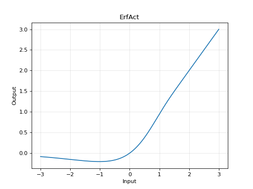
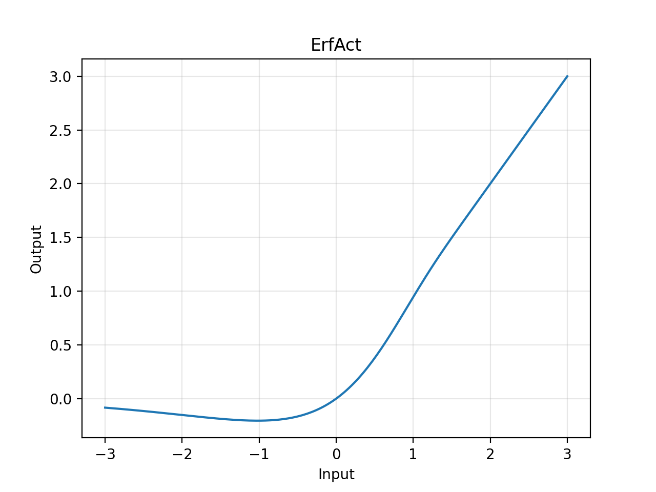
Apply the ErfAct activation function.
\[\text{ErfAct}(x) = x \cdot \text{erf}(a \cdot \exp(b \cdot x))\]- Parameters:
x (torch.Tensor) – Input tensor.
a (float, optional) – Scale parameter (default 0.5).
b (float, optional) – Exponent parameter (default 1.0).
- Returns:
The element-wise ErfAct of the input.
- Return type:
torch.Tensor
Source
See also
A variant of activation function using the error function, explored in “ErfAct and Pserf: Non-monotonic Smooth Trainable Activation Functions” (2022). arxiv
Example
import matplotlib.pyplot as plt
import torch

from activations_plus.simple import erf_act

x = torch.linspace(-3, 3, 200)
y = erf_act(x)
fig, ax = plt.subplots()
ax.plot(x.numpy(), y.numpy())
ax.set_title("ErfAct")
ax.set_xlabel("Input")
ax.set_ylabel("Output")
ax.grid(alpha=0.3)
fig.show()  # This will be mocked in tests
(
Source code,png,hires.png,pdf)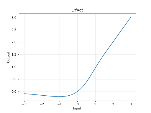
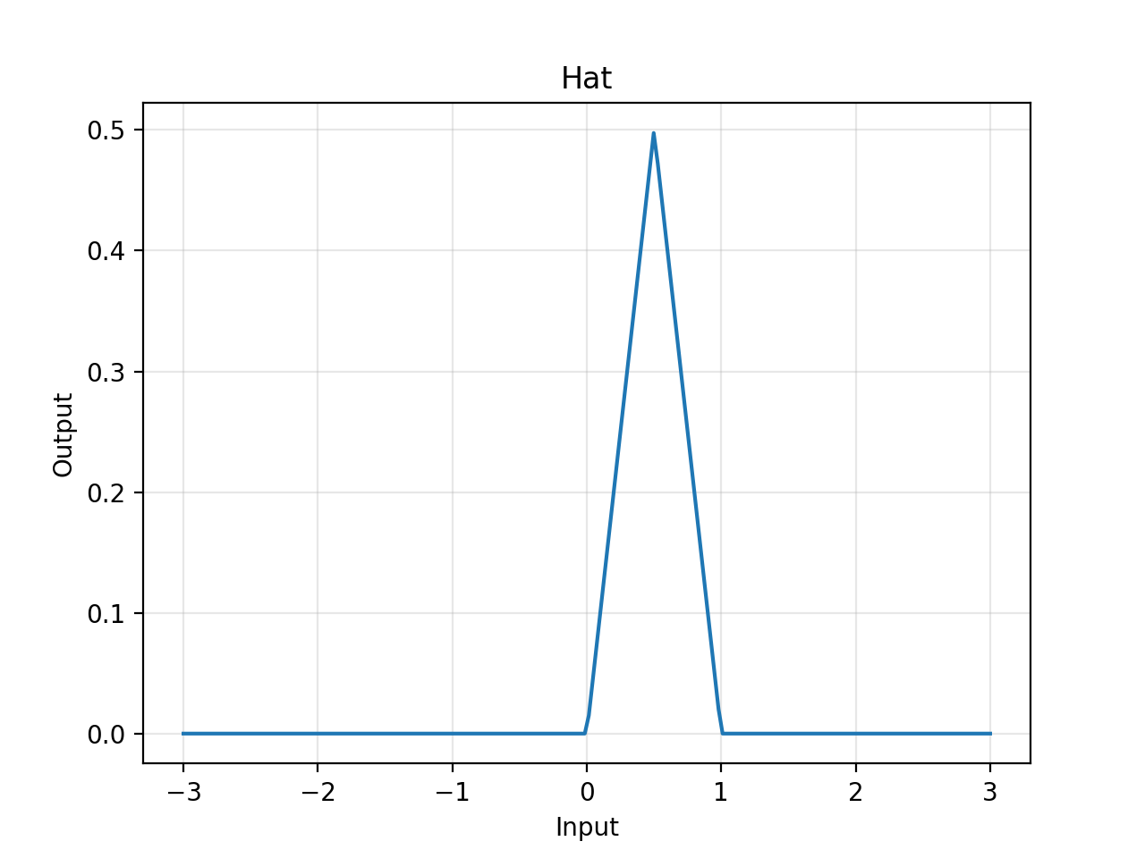
- activations_plus.simple.specialized_variants.hat(x: Tensor, a: float = 1.0) Tensor[source]
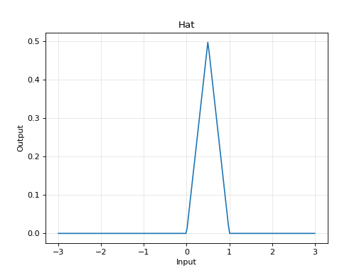
Apply the Hat activation function.
\[\begin{split}\text{Hat}(x) = \begin{cases} 0, & x < 0, \\ x, & 0 \leq x \leq \frac{a}{2}, \\ a - x, & \frac{a}{2} \leq x \leq a, \\ 0, & x > a, \end{cases}\end{split}\]- Parameters:
x (torch.Tensor) – Input tensor.
a (float, optional) – Hat width parameter (default 1.0).
- Returns:
The element-wise Hat function of the input.
- Return type:
torch.Tensor
Source
See also
Also known as triangular activation function, discussed in “On the Activation Function Dependence of the Spectral Bias of Neural Networks” (2022).
Example
import matplotlib.pyplot as plt
import torch

from activations_plus.simple import hat

x = torch.linspace(-3, 3, 200)
y = hat(x)
fig, ax = plt.subplots()
ax.plot(x.numpy(), y.numpy())
ax.set_title("Hat")
ax.set_xlabel("Input")
ax.set_ylabel("Output")
ax.grid(alpha=0.3)
fig.show()  # This will be mocked in tests
(
Source code,png,hires.png,pdf)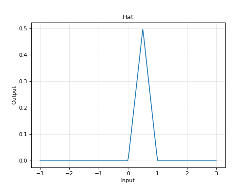
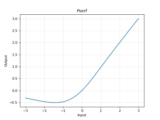
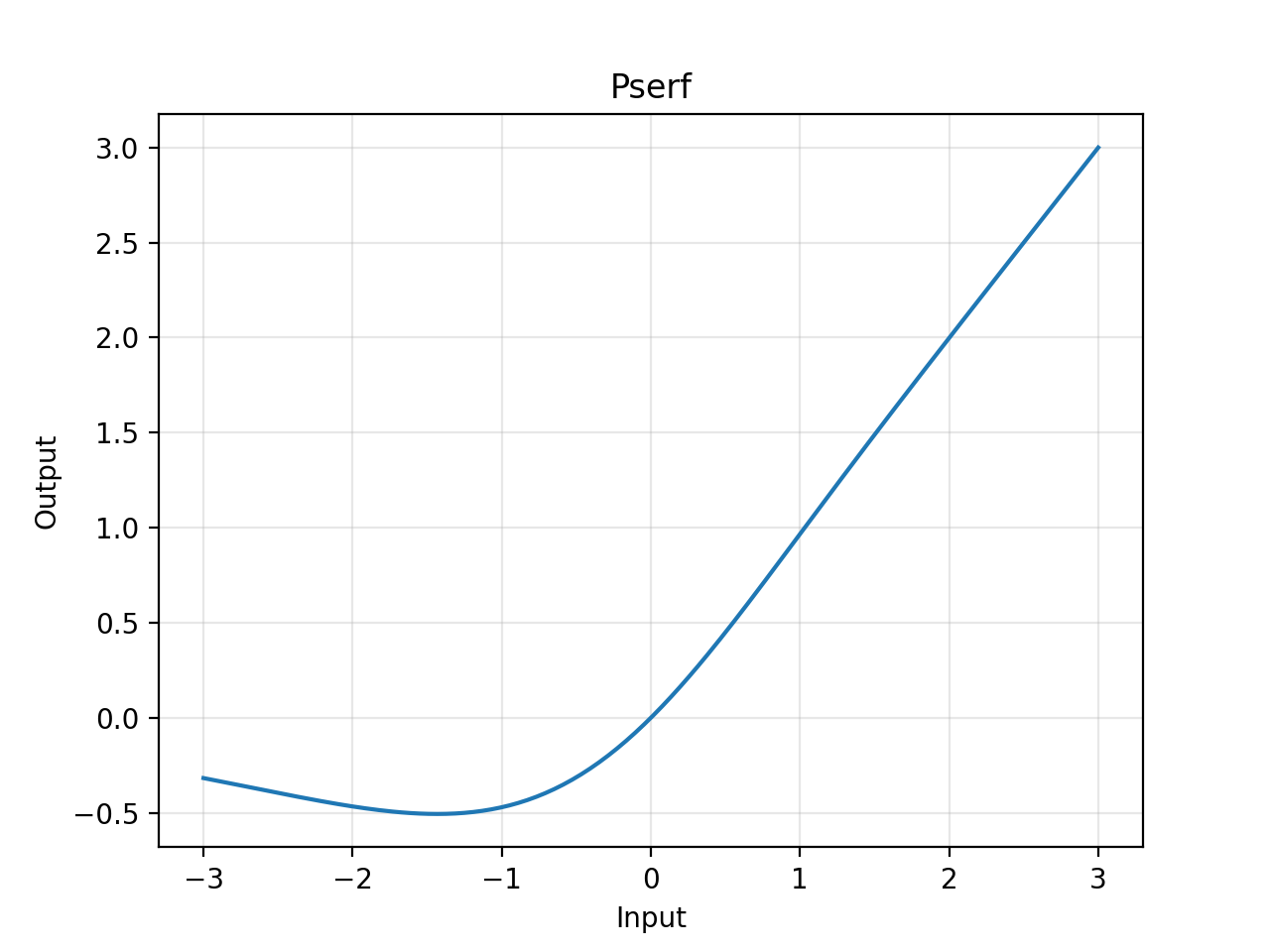
- activations_plus.simple.specialized_variants.pserf(x: Tensor, gamma: float = 1.25, delta: float = 0.85) Tensor[source]
Apply the Pserf (Parametric Serf) activation function.
\[\text{Pserf}(x) = x \cdot \text{erf}(\gamma \cdot \ln(1 + \exp(\delta \cdot x)))\]- Parameters:
x (torch.Tensor) – Input tensor.
gamma (float, optional) – Scale parameter (default 1.25).
delta (float, optional) – Exponent parameter (default 0.85).
- Returns:
The element-wise Pserf of the input.
- Return type:
torch.Tensor
Source
See also
A parametric version of the Serf activation function, introduced in “ErfAct and Pserf: Non-monotonic Smooth Trainable Activation Functions” (2022). arxiv
Example
import matplotlib.pyplot as plt
import torch

from activations_plus.simple import pserf

x = torch.linspace(-3, 3, 200)
y = pserf(x)
fig, ax = plt.subplots()
ax.plot(x.numpy(), y.numpy())
ax.set_title("Pserf")
ax.set_xlabel("Input")
ax.set_ylabel("Output")
ax.grid(alpha=0.3)
fig.show()  # This will be mocked in tests
(
Source code,png,hires.png,pdf)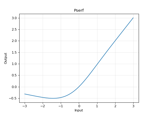
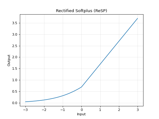
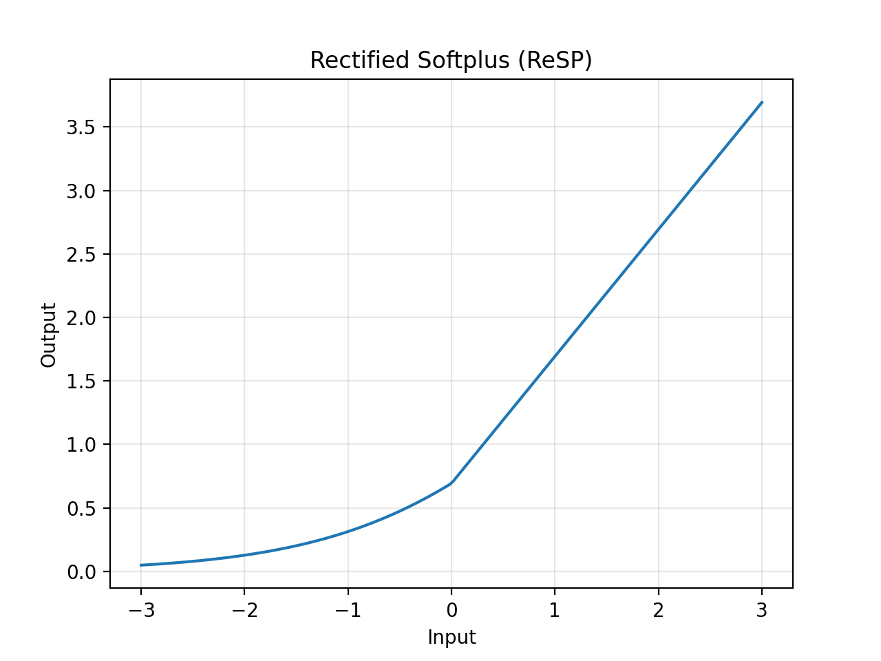
- activations_plus.simple.specialized_variants.resp(x: Tensor, a: float = 1.0) Tensor[source]
Apply the Rectified Softplus activation function.
\[\begin{split}\text{ReSP}(z) = \begin{cases} az + \ln(2), & z \geq 0, \\ \ln(1 + \exp(z)), & z < 0, \end{cases}\end{split}\]- Parameters:
x (torch.Tensor) – Input tensor.
a (float, optional) – Slope for positive inputs (default 1.0).
- Returns:
The element-wise ReSP of the input.
- Return type:
torch.Tensor
Source
See also
A combination of ReLU and softplus discussed in “Exploring the Relationship: Transformative Adaptive Activation Functions in Comparison to Other Activation Functions” (2024).
Example
import matplotlib.pyplot as plt
import torch

from activations_plus.simple import resp

x = torch.linspace(-3, 3, 200)
y = resp(x)
fig, ax = plt.subplots()
ax.plot(x.numpy(), y.numpy())
ax.set_title("Rectified Softplus (ReSP)")
ax.set_xlabel("Input")
ax.set_ylabel("Output")
ax.grid(alpha=0.3)
fig.show()  # This will be mocked in tests
(
Source code,png,hires.png,pdf)