Sigmoid and Tanh Variants

Sigmoid, tanh, and soft variants for PyTorch.

This module provides several simple sigmoid/tanh-based activation functions.

activations_plus.simple.sigmoid_tanh_variants.aria2(x: Tensor, alpha: float = 1.5, beta: float = 0.5) → Tensor[source]

Apply the ARiA2 activation function based on Richard’s curve.

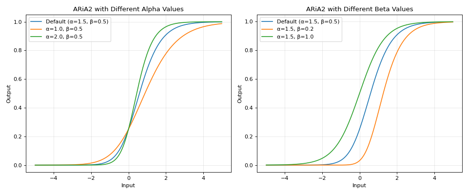
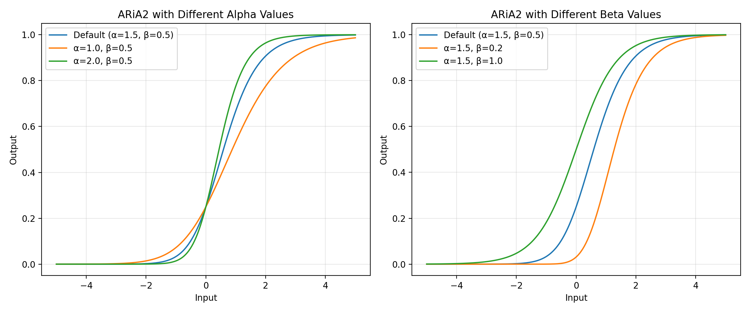
\[\mathrm{ARiA2}(z) = \frac{1}{(1 + e^{-\alpha z})^{1/\beta}}\]

Parameters:

x (torch.Tensor) – Input tensor.
alpha (float, optional) – Alpha parameter controlling the steepness (default 1.5).
beta (float, optional) – Beta parameter controlling the asymptotic behavior (default 0.5).

Returns:

The element-wise ARiA2 of the input.

Return type:

torch.Tensor

Source

See also

Introduced in “ARiA: Utilizing Richard’s Curve for Controlling the Non-monotonicity of the Activation Function in Deep Neural Nets” by Nader et al.

arxiv

Example

import matplotlib.pyplot as plt
import torch

from activations_plus.simple import aria2

x = torch.linspace(-5, 5, 200)

# Default parameters (alpha=1.5, beta=0.5)
y_default = aria2(x)

# Different alpha values
y_alpha_1 = aria2(x, alpha=1.0, beta=0.5)
y_alpha_2 = aria2(x, alpha=2.0, beta=0.5)

# Different beta values
y_beta_1 = aria2(x, alpha=1.5, beta=0.2)
y_beta_2 = aria2(x, alpha=1.5, beta=1.0)

fig, (ax1, ax2) = plt.subplots(1, 2, figsize=(12, 5))

# Plot different alpha values
ax1.plot(x.numpy(), y_default.numpy(), label="Default (α=1.5, β=0.5)")
ax1.plot(x.numpy(), y_alpha_1.numpy(), label="α=1.0, β=0.5")
ax1.plot(x.numpy(), y_alpha_2.numpy(), label="α=2.0, β=0.5")
ax1.set_title("ARiA2 with Different Alpha Values")
ax1.set_xlabel("Input")
ax1.set_ylabel("Output")
ax1.grid(alpha=0.3)
ax1.legend()

# Plot different beta values
ax2.plot(x.numpy(), y_default.numpy(), label="Default (α=1.5, β=0.5)")
ax2.plot(x.numpy(), y_beta_1.numpy(), label="α=1.5, β=0.2")
ax2.plot(x.numpy(), y_beta_2.numpy(), label="α=1.5, β=1.0")
ax2.set_title("ARiA2 with Different Beta Values")
ax2.set_xlabel("Input")
ax2.set_ylabel("Output")
ax2.grid(alpha=0.3)
ax2.legend()

plt.tight_layout()
fig.show()

(Source code, png, hires.png, pdf)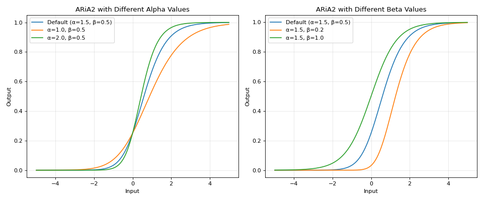

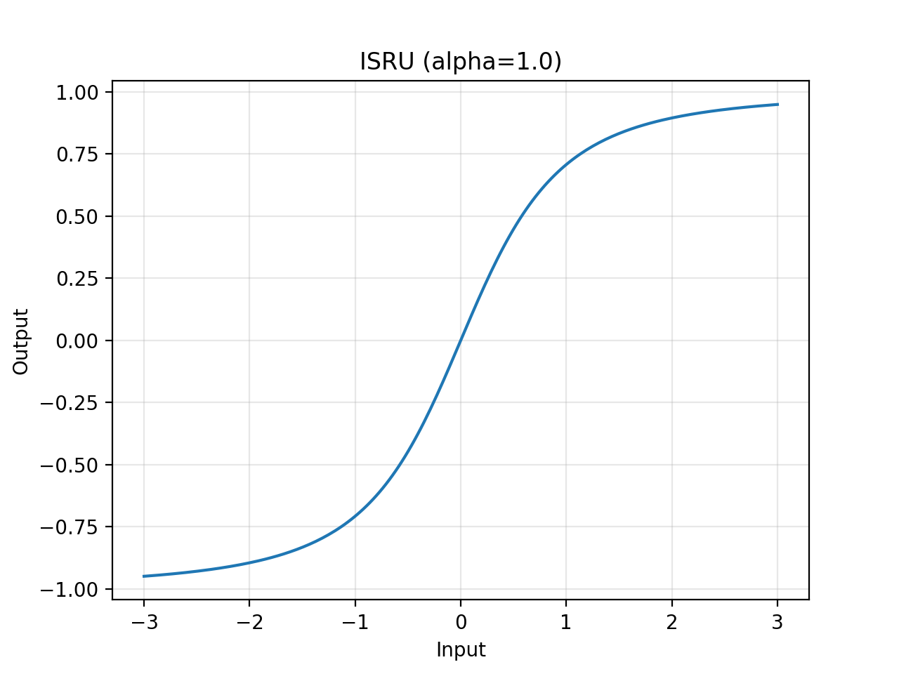
activations_plus.simple.sigmoid_tanh_variants.isru(x: Tensor, alpha: float = 1.0) → Tensor[source]

Apply the Inverse Square Root Unit activation function.

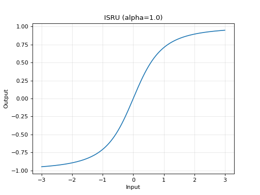
\[\text{ISRU}(z) = \frac{z}{\sqrt{1 + \alpha z^2}}\]

Parameters:

x (torch.Tensor) – Input tensor.
alpha (float, optional) – Scaling parameter (default 1.0).

Returns:

The element-wise ISRU of the input.

Return type:

torch.Tensor

Source

See also

Proposed in “Improving Deep Neural Networks with New Activation Functions” by Carlile et al. (2017).

arxiv

Example

import matplotlib.pyplot as plt
import torch

from activations_plus.simple import isru

x = torch.linspace(-3, 3, 200)
y = isru(x, alpha=1.0)
fig, ax = plt.subplots()
ax.plot(x.numpy(), y.numpy())
ax.set_title("ISRU (alpha=1.0)")
ax.set_xlabel("Input")
ax.set_ylabel("Output")
ax.grid(alpha=0.3)
fig.show()  # This will be mocked in tests

(Source code, png, hires.png, pdf)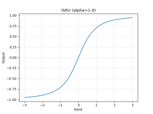

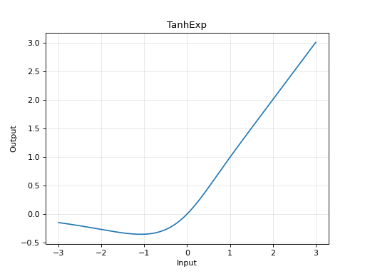
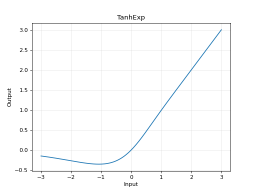
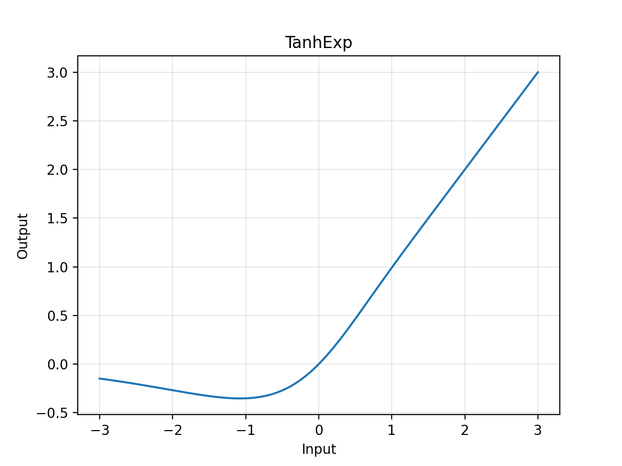
activations_plus.simple.sigmoid_tanh_variants.tanh_exp(x: Tensor, a: float = 1.0) → Tensor[source]

Apply the TanhExp activation function.

\[\text{TanhExp}(x) = x \tanh(\exp(x))\]

Parameters:

x (torch.Tensor) – Input tensor.
a (float, optional) – Scaling factor, default is 1.0.

Returns:

The element-wise TanhExp of the input.

Return type:

torch.Tensor